Trapezoid, Triangular, and Variable Load
This group of load types contains linearly variable distributed loads (LDL) along the element length or a part of it. The direction of loading can be specified in terms of either global or local coordinate directions.
The options Real length, Projection, Load/Unit length, Load mult. by CS width, Load mult. by CS depth and Nodal load are available as described for UDL.
This group of load types is limited to concentric loads (no eccentric load application).
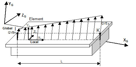
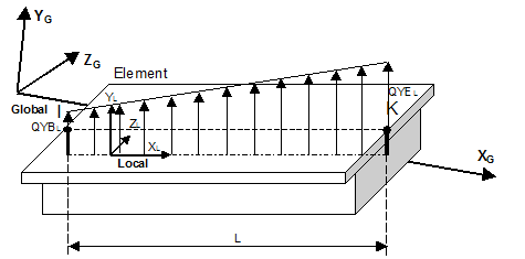
Trapezoidal element load – load types TG , TL
These types are used to define arbitrarily directed distributed loads with linearly variable intensity along the whole element length.
| Load Type | Description |
|---|---|
| TG | Trapezoidal LDL Global - Linearly variable distributed concentric element load (trapezoidal shape), specified by the load intensity components in global directions at the element begin (Qxb, Qyb, Qzb) and element end (Qxe, Qye, Qze). |
| TL | Trapezoidal LDL Local - Linearly variable distributed concentric element load, specified by the load intensity components in local directions at the element begin (Qxb, Qyb, Qzb) and element end (Qxe, Qye, Qze). |
Linear distributed moment load – load types QMG , QML
These types are used to define distributed moment loads with linearly variable intensity along the whole element length. The moments can either be defined in terms about global coordinate directions (QMG) or in terms of moment intensities about local directions (QML).
Positive moments are right-hand turning as shown in the figure for concentrated moments.
| Load Type | Description |
|---|---|
| QMG | Linearly variable distributed moment load, specified by the intensity values about global directions at the element begin (QMx-b, Qmy-b, QMz-b) and element end (QMx-e, QMy-e, QMz-e). |
| QML | Linearly variable distributed moment load, specified by the intensity values about local directions at the element begin (QMx-b, Qmy-b, QMz-b) and element end (QMx-e, QMy-e, QMz-e). |
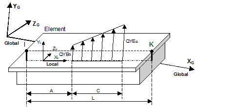
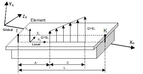
Partial trapezoidal element load – PTXG, PTXL, PTYG, PTYL, PTZG, PTZL
These types are used to define distributed loads with linearly variable intensity between a start and end point in an element. The start and end points are specified in terms of distances (A, C) from the element begin (currently no definition in terms of length related distances A/L, C/L).
| Load Type | Description |
|---|---|
| PTXG | Partial Trapezoidal LDL (X-direction Global). |
| PTXL | Partial Trapezoidal LDL (x-direction Local). |
| PTYG | Partial Trapezoidal LDL (Y-direction Global). |
| PTYL | Partial Trapezoidal LDL (y-direction Local). |
| PTZG | Partial Trapezoidal LDL (Z-direction Global). |
| PTZL | Partial Trapezoidal LDL (z-direction Local). |
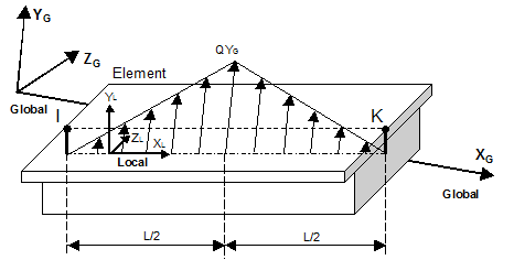
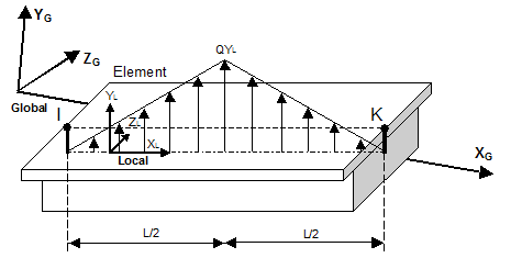
Triangular element load – load types DREIG, DREIL
| Load Type | Description |
|---|---|
| DREIG | Triangular element load (Global) – distributed concentric element load defined in the global coordinate system, with the load intensity raising linearly from 0 to Qx, Qy, Qz from both element ends to the element center. |
| DREIL | Triangular element load (Local) – distributed concentric element load defined in the local coordinate system, with the load intensity raising linearly from 0 to Qx, Qy, Qz from both element ends to the element center. |
Variable load along element – QVARNG, QVARNL, QVARLG, QVARLL, QVARXG, QVARXL, QVARYG, QVARYL, QVARZG, QVARZL
These load types are used to specify line loads arbitrarily distributed along an element or a series of elements. They have been provided for simulating wave loads acting on pile groups. Such wave loads have a special, partially curved, dependency on the depth below the water surface. However, these load types can be advantageously used for many other purposes, such as hydrostatic loading, earth pressure etc.
The direction of the loading is specified by entering the direction vector (DX, DY, DZ). This is either done in terms of global coordinate directions (option Global, load types QVARNG, QVARLG, QVARXG, QVARYG, QVARZG) or in terms of local directions (option Local, load types QVARNL, QVARLL, QVARXL, QVARYL, QVARZL). Note that the direction vector DX, DY, DZ is internally normalised to a length of 1.0 before being multiplied with the respective load intensity.
The options Real length and Projection can be used for relating the load to either the real element length or the projection of the element length as described for UDL.
The distribution of the load intensity must have been specified as an RM Bridge Variable (table!). This table is assigned in the GUI in the field Table. This table contains the load intensity as a function of an abscissa value, whose meaning is defined by selecting the appropriate option on the right side of the input pad:
- Option Element-normalized length the abscissa value is the normalized distance from the element begin (x/l).
- Option Element length the abscissa value is the actual distance from the element begin (local x coordinate).
- Option Element global X axis the abscissa value is the global x coordinate.
- Option Element global Y axis the abscissa value is the global y coordinate.
- Option Element global Z axis the abscissa value is the global z coordinate.
Such a table can also contain sections with curved shape, defined either by using a parabola interpolation or by specifying as ordinate value an expression dependent on the abscissa value tabA, as shown in the User Guide chapter 5.6.4, table 5-8. These arbitrary, maybe curved, distributions are modeled as piecewise linear, internally using the partial trapezoidal load types described in the preceding sections. In order to increase accuracy or to decrease computing time, the user can change the number of linear pieces per element (parameter Ntel) being per default set to 16.
Special applications may require using a cover function for assigning different tables to different elements. This cover function will be a table containing the actual distribution table names as ordinates, dependent on an internal variable IQVAR as abscissa value (e.g., IQVAR=1→TableA, IQVAR=2→TableB, etc.). The name of the cover function will be specified in the input field Table, and depending on the current value of IQVAR the appropriate distribution table will be taken.
The parameters I-Var1 and I-Var2 are used for calculating the variable IQVAR for the nth element in the specified element series as function n: IQVAR = I-Var1 + (n-1)×I-Var2.