G.17.3.5 Response Time History
STAAD.Pro is equipped with a facility to perform a response history analysis on a structure subjected to time varying forcing function loads at the joints and/or a ground motion at its base. This analysis is performed using the modal superposition method. Hence, all the active masses should be modeled as loads in order to facilitate determination of the mode shapes and frequencies. Refer to G.17.3.2 Mass Modeling for additional information on this topic. In the mode superposition analysis, it is assumed that the structural response can be obtained from the "p" lowest modes. The equilibrium equations are written as
[m]{x''} + [c]{x'} + [k]{x} = {P(t)}
Using the transformation
The equation for {P(t)} reduces to "p" separate uncoupled equations of the form
| q''i + 2 ξiωiq'i + ωi2qi = Ri(t) |
| = | ||
| = |
These are solved by the Wilson- θ method which is an unconditionally stable step by step scheme. The time step for the response is entered by you or set to a default value, if not entered. The qis are substituted in equation 2 to obtain the displacements {x} at each time step.
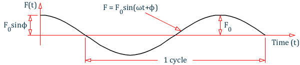
Time History Analysis for a Structure Subjected to a Harmonic Loading
| F(t) = F0sin(ωt + ϕ) |
| = | ||
| = | ||
| = | ||
| = |
The results are the maximums over the entire time period, including start-up transients. So, they do not match steady-state response.
Definition of Input in STAAD.Pro for the above Forcing Function
As can be seen from its definition, a forcing function is a continuous function. However, in STAAD.Pro, a set of discrete time-force pairs is generated from the forcing function and an analysis is performed using these discrete time-forcing pairs. What that means is that based on the number of cycles that you specify for the loading, STAAD.Pro will generate a table consisting of the magnitude of the force at various points of time. The time values are chosen from this time '0' to n*tc in steps of "STEP" where n is the number of cycles and tc is the duration of one cycle. STEP is a value that you may provide or may choose the default value that is built into the program. STAAD.Pro will adjust STEP so that a 1/4 cycle will be evenly divided into one or more steps. See TR.31.4 Definition of Time History Load for a list of input parameters that need to be specified for a Time History Analysis on a structure subjected to a Harmonic loading.
The relationship between variables that appear in the STAAD.Pro input and the corresponding terms in the equation shown above is explained below.
- F0 = Amplitude
- ω = Frequency
- ϕ = Phase
Forces applied at slave dof will be ignored; apply them at the master instead.